Correcting Coherent Errors with Surface Codes

Update (31.10.18): This project was recently published in Nature!

This is a paper that resulted from a project I assisted with during a summer internship with the group of Robert König at TU München. I was responsible for writing efficient C++ code to simulate the algorithms proposed in the paper. I cannot claim to understand all of the mathematics involved but I thought the code I wrote worked pretty well. I was also grateful for the opportunity to sample the academic environment in Germany.

Here is a link to our paper on the arXiv. The abstract is copied below.

"We study how well topological quantum codes can tolerate coherent noise caused by systematic unitary errors such as unwanted Z-rotations. Our main result is an efficient algorithm for simulating quantum error correction protocols based on the 2D surface code in the presence of coherent errors. The algorithm has runtime O(n2), where n is the number of physical qubits. It allows us to simulate systems with more than one thousand qubits and obtain the first error threshold estimates for several toy models of coherent noise. Numerical results are reported for storage of logical states subject to Z-rotation errors and for logical state preparation with general SU(2) errors. We observe that for large code distances the effective logical-level noise is well-approximated by random Pauli errors even though the physical-level noise is coherent. Our algorithm works by mapping the surface code to a system of Majorana fermions."

Water Molecular Dynamics - Some Graphs

I made these plots a few years ago for a class on quantum chemical simulation at MIT; I still find them interesting to look at sometimes. These plots were produced from a molecular dynamics simulation with magnesium chloride in an explicit water solvent using various water models such as TIP3P/TIP4P and SPCFW.

You will notice that the quantities plotted below have wildly fluctuating raw data due to the small number of explicit solvent molecules present in the simulation. How is this useful? The point here is that the averages of these quantities stabilize and reach equilibrium by the end of the simulation. Molecular dynamics simulations frequently makes use of the ergodic hypothesis in this way.

Each plot includes the raw data, a smoothed version of the raw data, and a cumulative average. For experimentalists, it is usually only the average at the end of simulation that is important as this is assumed to be the equilibrium value of the measured quantity.

Water density (no solute) over time in the SPCFW model.

Water temperature (no solute) over time in the SPCFW model.

Water temperature (no solute) over time in the SPCFW model.

Radial probability distribution of water molecules around magnesium and chloride ions in solution. Note the secondary water shell of magnesium.

Distance between magnesium ion and both accompanying chloride ions over time in solution. 

Heilmeier's Catechism

This is a set of questions that I was unaware of until one of my professors at MIT mentioned it in a class. It's a good rubric for any project and I'm not sure why it is not more commonly known. Or perhaps it is and I'm just the last person to learn about it.

From the Wikipedia page: A set of questions credited to George H. Heilmeier that anyone proposing a research project or product development effort should be able to answer.

• What are you trying to do? Articulate your objectives using absolutely no jargon.
• How is it done today, and what are the limits of current practice?
• What's new in your approach and why do you think it will be successful?
• Who cares? If you're successful, what difference will it make?
• What are the risks and the payoffs?
• How much will it cost?
• How long will it take?
• What are the midterm and final "exams" to check for success?

Good questions to come back to on any serious project or research.

Mathematica Basic Functions and Examples

Reading software documentation is boring and Mathematica is a pain so here are some examples of the key functions and their syntax just to get started. I will attempt to update this in the future although I try to find alternatives to Mathematica whenever possible.

# Integration
Integrate[2*Sqrt[2]/(3*a)*x*Sin[2*Pi*x/a]*Sin[3*Pi*x/a], {x, 0, a}]

# Numerical Integration
N[Integrate[4/a^3*r^2*Exp[-2 r/a], {r, 0, a/53600}]]

# Integration over multiple dimensions
Integrate[1/(2*u)*(Q*w*u/(4*Pi*R))^2*((1 - 3*r^2/(5*R^2))^2*Cos[t]^2 + 
(1 - 6*r^2/(5*R^2))^2*Sin[t]^2)*r^2*Sin[t], {t, 0, Pi}, {p, 0, 2 Pi}, {r, 0, R}]

# Finding Intersections
pts = NSolve[x*Cot[x] == -y*Coth[y] && {x, y} \[Element] Circle[{0, 0}, 2*Pi], {x, y}]

# A plot of the above intersections
ContourPlot[{x*Cot[x] + y*Coth[y] == 0 , x^2 + y^2 == 4 Pi^2}, 
{x, -4 Pi, 4 Pi}, {y, -4 Pi, 4 Pi}]

# The Quantum Harmonic Oscillator and some expectation values
Clear[m, \[Omega], \[HBar], n];
(*m=1*)
(*\[Omega]=1*)
(*\[HBar]=1*)

psi[x_, n_] := (m*\[Omega]/(Pi*\[HBar]))^(1/4)*1/Sqrt[2^n*n!]*
  HermiteH[n, Sqrt[m*\[Omega]/(\[HBar])]*x]*
  Exp[-m*\[Omega]*x^2/(2*\[HBar])]
En[n_] = \[HBar]*\[Omega]*(n + 1/2)
En[0]
psi[x_, t_, n_] := (m*\[Omega]/(Pi*\[HBar]))^(1/4)*1/Sqrt[2^n*n!]*
  HermiteH[n, Sqrt[m*\[Omega]/(\[HBar])]*x]*
  Exp[-m*\[Omega]*x^2/(2*\[HBar])]*Exp[-i*En[n]*t/\[HBar]]
psi[x, 0]
psi[x, t, 0]
expX[n_] := Integrate[x*psi[x, n]^2, {x, -Infinity, Infinity}]
expX2[n_] := Integrate[x^2*psi[x, n]^2, {x, -Infinity, Infinity}]
DeltaX[n_] := Sqrt[expX2[n] - expX[n]^2]

# Expand expressions
Expand[Sum[
  1 + e^(I*(Subscript[K, 3] - Subscript[K, 1]) (Subscript[x, i] - 
        Subscript[x, k])) + 
   e^(I*(Subscript[K, 1] - Subscript[K, 2]) (Subscript[x, j] - 
        Subscript[x, i])) + 
   e^(I*(Subscript[K, 2] - Subscript[K, 3]) (Subscript[x, k] - 
        Subscript[x, j])) + 
   e^(I*(Subscript[K, 1]*(Subscript[x, j] - Subscript[x, i]) + 
        Subscript[K, 2]*(Subscript[x, k] - Subscript[x, j]) + 
        Subscript[K, 3]*(Subscript[x, i] - Subscript[x, k]))) + 
   e^(I*(Subscript[K, 1]*(Subscript[x, k] - Subscript[x, i]) + 
        Subscript[K, 2]*(Subscript[x, i] - Subscript[x, j]) + 
        Subscript[K, 3]*(Subscript[x, j] - Subscript[x, k]))), {i, 
   n}, {j, n}, {k, n}]]

# Simplify expressions, '%' uses the result of the previous input
FullSimplify[%]

A couple key differences to note about Mathematica: The use of square brackets instead of parentheses to contain arguments to functions, function names are capitalized, comments are indicated by '(*' and a closing '*)', and user-defined functions are created using ':=' and underscores on any arguments. If possible, I encourage use of open source alternatives such as Octave or Python. However, I have to admit that, when it comes to getting integration and algebra of complicated expressions done quickly, nothing beats Mathematica.

Using Wine for Gaming in OSX - SWTOR

I like Star Wars and sometimes I feel compelled to revisit the games from my youth; however, this can be a bit difficult when one uses OSX (though there are some excellent ports of the classics, and other favorites, from Aspyr Media on the App Store). Wine, again, proves to be very useful in this area even for the MMORPG Star Wars The Old Republic at the highest graphics settings.

Setup for this game requires some patience but not nearly so much as it used to be when the clues were more scattered a few years ago (plus there are fewer steps required now, for a number of reasons). This guide on reddit is kept up-to-date and is very comprehensive but I'll describe what I did for reinforcement.

Download the latest Wine Staging version. I have had problems trying to use MacPorts to install Wine so I recommend downloading the installer from the website directly. 

Open a Terminal using your Wine install. Use "winecfg" to set Windows 10, and include d3dx9_43, crypt32. Remember, the default is that all Wine related items are stored in a mock Windows-style directory tree in ~/.wine. This is where all of the SWTOR files will be installed.

Download and run the SWTOR installer with Wine. I have only tested the "Express" install and had no issues with this step.

Run the SWTOR launcher by changing into the install directory under ~/.wine. Then, login to your account. At this point, an error will popup saying something about administrative privileges. Close the launcher. Open launcher.settings using a text editor and change the line "bitraider_disable": false to "bitraider_disable": true.

Run the launcher again. Login and allow the game to patch. Expect this to take several hours depending on your connection. The full game is 38 GB on the hard drive so make sure you can afford the space.

Screen shot of launcher window on OSX

Once you are fully patched, that should be it. I have played the game a couple of times since installing and it runs well even over WiFi on the highest graphics settings. I'm sure using Wine to run other Windows games on OSX would work well too. My MacBook has an AMD Radeon R9 M370X in addition to the integrated Intel Iris Pro so your mileage may vary on your own system. 

May the Force be with you.

Compiling BoltzTraP 1.2.5 on OSX

Update (21.6.18): I've noticed in using BoltzTraP2 that it has much greater numerical stability than previous versions of BoltzTraP. I must conclude that BoltzTraP2 gives much more reliable results. Reproducing the band structure near band crossings, as I mentioned previously, may be failing due to insufficient k-point sampling in terms of overall density at specific locations in k-space that are required to resolve the bands near a crossing.

Update (19.6.18): I was not unaware of BoltzTraP2, but I was skeptical of the new version at first (and I was determined to get 1.2.5 working again). Turns out, it works rather well and is easy to use without the need to write custom scripts for converting or processing data from an electronic structure code output. It also allows interactive plotting of the entire Fermi Surface which is a fun feature. The transport coefficients calculated are nearly identical to those calculated in version 1.2.5 and the built-in plotting feature facilitates plotting over a range of temperatures.

Fermi surface of silicon as calculated from VASP in BoltzTraP2. 

Another section of the silicon Fermi surface.

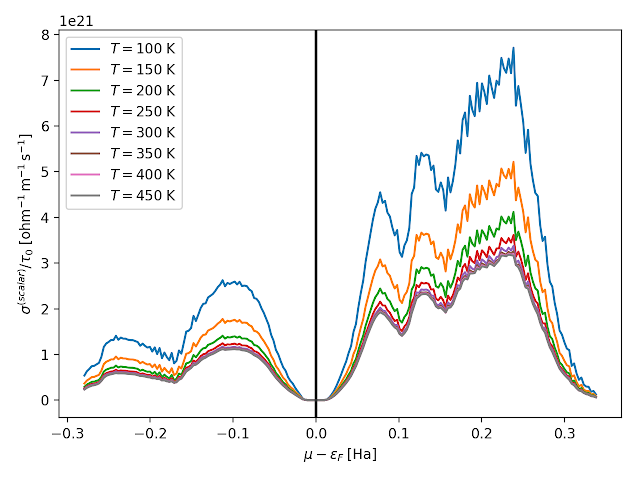
Conductivity of silicon as a function of chemical potential at various temperatures as calculated in BoltzTraP2.

Conductivity of silicon as calculated in BoltzTraP 1.2.5. Roughly corresponds to the region between -0.1 and 0.1 Hartrees in the previous plot. The point is just to show that the main features are reproduced with identical orders of magnitude.

The plotting tool is not, however, great for plotting band structures: It does not give the smooth plots that can be made in Python and often gets confused near band crossings. I suspect that this is probably an issue with the plotting function itself and not due to the interpolation, which the BoltzTraP team claimed in their original paper sufficiently approximated the band structure near band crossings for the purpose of calculating the transport coefficients.  

Band structure of silicon from VASP plotted using custom data processing and scripts.

Band structure of silicon plotted by BoltzTraP2 across the same high symmetry points as in the previous plot. Note here, however, that the features are not reproduced with the same resolution nor even with the same accuracy near band crossings. BoltzTraP2 does give a rough idea of the features but clearly it is necessary to do a full band structure calculation with explicit k-point path in VASP rather than interpolate a uniform k-point density DOS calculation as BoltzTraP2 does. 

Follow this tutorial for more information. I tested it using VASP calculations on silicon and had no problems.

Original: I recently had some trouble getting BoltzTraP to compile and play nicely with MacPorts so I am posting the final results. It is the upper section of the Makefile that is most important but I have included the entirety for completion. I used MacPorts' gfortran, lapack (+gfortran), and scalapack (+gfortran). It proved important to not let the compiler or linker find any ATLAS libraries or OSX's Accelerate framework: If you have ATLAS installed through MacPorts, there will be a liblapack.a in /opt/local/lib that belongs to ATLAS. The Makefile below correctly tells the linker to use /opt/local/lib/lapack instead.

# BoltzTraP 1.2.5 Makefile

SHELL = /bin/sh
FC = /opt/local/bin/gfortran
FOPT  = -g -funroll-loops -O3 -ffast-math -fgcse-lm -fgcse-sm -ffast-math \
-ftree-vectorize -fexternal-blas -fleading-underscore -g -p -pg -Wall \ 
-fbounds-check -finit-integer=-666 -finit-real=nan

LDFLAGS = -L/opt/local/lib/lapack -L/opt/local/lib/
LIBS = -lblas -lscalapack -llapack

LINKER = $(FC)
DESTDIR = .
EXECNAME = BoltzTraP

###############################################################################

FFLAGS = $(FGEN) $(FOPT)
EXEC = $(DESTDIR)/$(EXECNAME)

#..............................................................................
#
#  Object files common to both REAL and COMPLEX type subroutines
#
OBJS = gmlib2.o reallocate.o \
     m_bandstructure.o m_input.o m_fermimod.o \
     m_interfaces.o \
     latgen2.o generic_field.o gtfnam.o gen_lattpoints.o \
     BoltzTraP.o crystal_band.o wien_band.o phon_band.o generic_band.o pw_interface.o \
     add_inv.o bandana.o stern1.o kdelta.o fite4.o sortag.o gplbands.o \
     dos.o ifflim.o setfft.o c3fft.o boseintegrals.o fermiintegrals.o bands.o kcomp.o \
     bz.o fermisurface.o setfft2.o write_dx_fs.o write_dx_bz.o write_cube_fs.o \
     dos_histogram.o dos_tetra.o noculc.o dosvv.o readvv.o \
     phonondrag.o
#OBJS = \
#        reallocate.o defs.o modules.o broad.o add_inv.o \
#        c3fft.o gtfnam.o ifflim.o mknam.o read_energy.o \
#        transport.o stern.o kdelta.o gen_lattpoints.o fite4.o setfft.o \
#        starfkt2.o dos.o 

$(EXEC): $(OBJS)
 $(LINKER) $(LFLAGS) -o $(EXEC) $(OBJS) $(LDFLAGS) $(LIBS) $(LFLAGS)


clean:
 rm -f *.o *.mod *.pc *.pcl *~

.SUFFIXES: .F90 .o 
.F90.o:
 $(FC) $(FFLAGS) -c $<