Since this class of problem has come up in multiple of my quantum physics courses at MIT, I think it is worthwhile to work through an example here and show the relevant steps in Mathematica (arguably, the most difficult part and certainly the most frustrating). Using this work flow, we should be able to find the eigenvalues of any one-dimensional potential we choose.
Let's use the one-dimensional potential \(V(x) = \alpha x^4\). We consider the time-independent Schrödinger equation, $$\frac{-\hbar^2}{2m} \frac{d^2}{dx^2} \psi + \alpha x^4 \psi = E \psi(x)$$ To make this equation dimensionless, we can perform a change of variable with \(x=\beta u\). \(x\) has units of length so, to express it in terms of a dimensionless parameter, we say that \(\beta\) is some constant parameter with whatever units of length we like (picometers, kilometers, lightyears, etc.) and \(u\) is a continuous dimensionless parameter (i.e., a number). Since \(\beta\) is constant, we can express the Schrödinger equation in terms of \(u\), our dimensionless parameter (note how \(u = x/\beta \) has no units). This is what is meant when we say that we want to make the Schrödinger equation dimensionless. It seems like a silly or pointless trick (at least, I thought so at first) but it really does make working with differential equations much simpler; this is especially true if we want to solve physical differential equations on a computer, since making a computer understand dimensional analysis is a much larger programming task than we would like to do just to solve a single ordinary differential equation.
Using the substitution \(x=\beta u\), we can rewrite the Schrödinger equation above as $$\frac{-1}{2} \frac{d^2}{du^2}\psi + (u^4-e)\psi = 0$$ after setting $$\beta = \left(\frac{\hbar^2}{m \alpha}\right)^\frac{1}{6}$$ and noting that $$ \frac{d^2}{dx^2}\psi = \frac{1}{\beta^2} \frac{d^2}{du^2} \psi \qquad e = \left( \frac{m^2}{\hbar^4 \alpha} \right)^\frac{1}{3} E $$ Note, also, that the \(\psi\) in the dimensionless equation and the \(\psi\) in the previous equation are different: One is in terms of \(x\) and the other in terms of \(u\). But, since we are only interested in finding the ground-state energy, for the purposes of this example we only care that we have found a simple relation between \(E\) and dimensionless \(e\). (We could, if we were solving this analytically, find an expression for \(\psi(u)\) and transform to \(\psi(x)\) by inserting \(\beta\) where appropriate.)
With our dimensionless expression for the Schrödinger equation and a valid relation between \(E\) and dimensionless parameter \(e\), we are ready to plug this into Mathematica. We need to select valid initial conditions for the ground-state wave function. Since this is an attractive potential and we are searching for the ground-state energy, we know that the wave function should have no nodes and be normalizable. Since the potential we have chosen is symmetric, we can assert that the ground state must have \(\psi'(0) = 0\) and \(\psi(0) = 1\) (choosing \(\psi(0) = 1\) rather than any other non-zero value is arbitrary, since we could always normalize the wave function). We can plug this information into Mathematica's ParametricNDSolve, which will solve the differential equation numerically in terms of the parameter \(e\).
pfun = ParametricNDSolveValue[{-0.5*psi''[u] + (u^4 - e)*psi[u] == 0,
    psi[0] == 0, psi'[0] == 1}, psi, {u, -30, 30}, {e}];
Plot[Evaluate@Table[pfun[e][x], {e, 0, 1, 0.1}], {x, -10, 10}]Plot[pfun[e][10], {e, 0, 8}]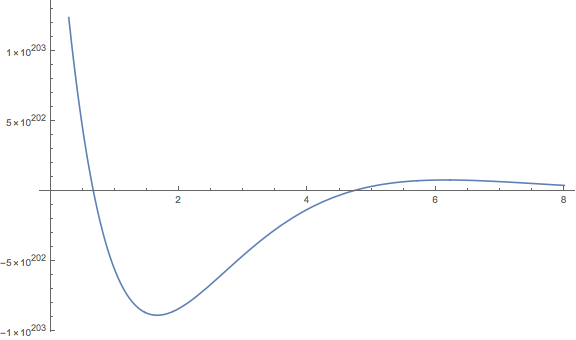
Plotting reveals that \(\psi(u=10, e)\) does cross the x-axis, minimizing \(\psi\) for large \(u\) at certain values of \(e\). The first such \(e\) should be our ground-state dimensionless energy. We can use FindRoot in Mathematica to determine the crossing-point to arbitrary precision. Once we find a value for \(e_0\) we can easily find \(E_0\) using our relation from before.
val = Map[FindRoot[pfun[e][10], {e, #}, WorkingPrecision -> 20] &, {2}]These types of problems used to be particularly annoying in my MIT courses because the suggested method by the instructors was to search for the optimal value of \(e\) (to six decimal places!) by manually inputting values. Lots of time wasted because not everyone knew how to use Mathematica or of the existence of ParametricNDSolve.
The complete Mathematica code to solve this problem is copied below.
Clear[e]
pfun = ParametricNDSolveValue[{-0.5*psi''[u] + (u^4 - e)*psi[u] == 0,
    psi[0] == 0, psi'[0] == 1}, psi, {u, -30, 30}, {e}];
Plot[Evaluate@Table[pfun[e][x], {e, 0, 1, 0.1}], {x, -10, 10}]
Plot[pfun[e][10], {e, 0, 8}]
val = Map[FindRoot[pfun[e][10], {e, #},  WorkingPrecision -> 20] &, {2}]

