Building ATLAS in Mac OSX

The Automatically Tuned Linear Algebra Software (ATLAS) is a popular implementation of the Basic Linear Algebra Subroutines (BLAS) and some LAPACK routines. Such modules are commonly used to speed-up computations in scientific applications that require many and fast matrix operations. Below, I will demonstrate how to build ATLAS in OSX on a MacBook Pro (2015).

For comparison, below are my system specifications.

Modellname:                MacBook Pro
Modell-Identifizierung:    MacBookPro11,5
Prozessortyp:              Intel Core i7
Prozessorgeschwindigkeit:  2,8 GHz
Anzahl der Prozessoren:    1
Gesamtanzahl der Kerne:    4
L2-Cache (pro Kern):       256 KB
L3-Cache:                  6 MB
Speicher:                  16 GB
Systemversion:             macOS 10.13.4
Kernel-Version:            Darwin 17.5.0

To begin, download ATLAS. The latest stable version is 3.10.3 as of writing and this is the version I tested. However, even this latest stable release is dated by about two years (as of 2018) so you might consider trying one of new developer versions of find an alternative to ATLAS that is more actively managed.

Place the tar files in your home directory. Extract the ATLAS tar file using the command below.

tar -xvf atlas3.10.3.tar.bz2

Create a build subdirectory under the ATLAS directory that the tar files were extracted to.

mkdir build
cd build

At this point, make sure that you have a functioning gcc and gfortran compiler. Use Homebrew to install the gcc8 compiler (gfortran is included in gcc8). Type "gfortran" to verify it is working. You need to mess around with aliases or your path variable to compile with gcc, but we will force ATLAS to use clang below.

(Warning: I've tried many times to get this install process working with MacPorts and the compilers it provides without success. I believe this is because the compilers installed by MacPorts were not working nicely with each other or the XCode command line tools. Save yourself some time and use a clean install of Homebrew and the latest gcc.)

From the build directory, run the configure script. You can have ATLAS build a full LAPACK library by downloading a LAPACK tarfile from NetLib and using "--with-netlib-lapack-tarfile=path/to/tarfile" in the configure step, but this is optional.

../configure -A Corei3 -b 64 -D c -DI7CPS=2800 --prefix=/app/atlas3.10.3/build --force-clang=/usr/bin/clang --with-netlib-lapack-tarfile=/app/lapack-3.8.0.tar.gz

Double check the Make.inc file in the build directory for anything unusual. In particular, ATLAS may be unable to detect your chip architecture. I fixed this by adding -A Corei3 to the above command, but double check for your system.

Before building ATLAS, if possible, find a method to disable CPU throttling on OSX as this will disrupt ATLAS's timings which it uses to tune the BLAS to the hardware. There are some suggestions for how to do this on the Web but just as many suggestions say this is not possible for some i7 processors since CPU throttling is done "on-the-fly" in hardware. The solutions I have attempted have had no effect on the quality of the ATLAS build that I can discern.

Once you are ready to build, make sure your device is attached to a power source and all other processes are idle. The build and testing could take several hours, depending on which compiler you chose, and generate a lot of heat. It may be convenient to do this overnight. Enter make build to begin building ATLAS.

make build

The build process will send many hundreds of pages of output to the terminal. This is normal. Keep waiting. If you used the clang compiler, this should not take so long. After this point, if you want to change any of the configuration settings and recompile, it is best to delete the whole build directory and start over to avoid confusing compilation errors.

Once the build has completed, check for any obvious errors in the last several pages of output from the compiler. Then start running the following tests. The full test is only necessary for further debugging if you see weird things in the check and parallel check sections.

make check

make ptcheck

make full_test

Finally, run the timing and install.

make time

make install

The compiled ATLAS library will be in /ATLAS/build/lib/libatlas.a. Link to this library when compiling other programs like Quantum Espresso.

A summary of the necessary commands.

# Place the ATLAS tar file in the home directory

tar -xvf atlas3.10.3.tar.bz2
cd ATLAS
mkdir build
cd build 

/Users/localuser/ATLAS/configure -A Corei3 -b 64 -D c -DI7CPS=2800 --prefix=/Users/nolanpeard/ATLAS/build --force-clang=/usr/bin/clang

make build
make check
make ptcheck
make time
make install

References:
ATLAS
BLAS
LAPACK
ScaLAPACK

CdSe Quantum Dot Photos

Today, I attempted to replicate the results of this paper in an experimental physics class at MIT. I asked some of my graduate student friends and eventually found someone in a chemistry group who was willing to give me a small sample of CdSe quantum dots with 625 nm emission. Unfortunately, the experiment did not work in our optical trap in the time I had to test it and I had to abandon the project. (I think our trapping laser was not powerful enough to access the two-photon absorption process. The photodetector was probably not sensitive enough either.)

I did, however, take some nice photos of the fluorescing quantum dots. I used a 405 nm flashlight to excite the dots. I noticed they will even fluoresce a tiny amount from indirect sunlight on a cloudy day.

CdSe quantum dots in hexane with no excitation.

CdSe quantum dots excited with a 405 nm flashlight. Fluorescence should be about 625 nm.

Multigrain Bread Recipe

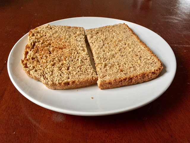
Read to the end of the article for an improved recipe. For the original recipe, courtesy of my grandmother, combine the ingredients in order as listed. 

• Multigrain cereal, 1 cup 
• Boiling water, 1.5 cup
• Vegetable oil, 3 tablespoons 
• Honey, 4 tablespoons 
• Bread flour, 3 cups 
• Salt, 1 teaspoon 
• Gluten, 1 tablespoon 
• Toasted wheat germ, 2 tablespoons 
• Flax seed, 2 tablespoons 
• Yeast, 2 teaspoons

The boiling water is intended to soften the multi-grain cereal but must be allowed to cool completely before adding further ingredients. Yeasts do not like extreme temperatures!

I've been making this recipe in my bread machine for about two years and, though it does work, there are some recurring issues: the bread often struggles to rise completely and is very crumbly. The unpredictability of the rise was particularly frustrating and I began experimenting to find a solution. It has taken almost a year and some careful reading of Whole Grain Breads by Peter Reinhart, but I believe I have now found a superior recipe that rises consistently and is marginally less crumbly. 

The key modifications are to use cold instead of boiling water, add one egg, and use much more gluten. (I also add a cup of oats and an extra half-cup of water but this is probably not necessary.) There are a few reasons why this gives a better rise. First, using cold tap instead of boiling water does not kill off any natural yeasts in the cereal or other ingredients. The grains will not soften as quickly but I've never noticed a difference in the finished product since the grains soften during baking anyway. Second, adding an egg helps all of the grains stick together by adding protein. The extra gluten is used for the same purpose. Proteins polymerize during kneading to form a cohesive network that traps the gases released by the yeast; if there is not enough protein/gluten in the recipe the gases escape and bread fails to rise. This is, in fact, why there is a distinction between bread flour and other types of flour: Bread flour tends to have a higher percentage of protein that helps the bread rise better. Adding sticky proteins also helps to make the bread less crumbly.

Having enough gluten and other protein in the dough is particularly crucial for multigrain breads because they have so many large, partially-milled grains. Large particles simply do not stick together as readily as small particles. Additionally, the large grains can be very sharp (just examine a flax seed carefully) from the perspective of the polymeric proteins; they act like tiny blades on the polymer chains during kneading, creating holes and allowing precious gas to escape. This is why I have to take care to add extra gluten if I want to substitute some of the bread flour with whole wheat flour.

Another set of parameters to pay attention to during troubleshooting is the amount of water and salt. Yeast needs plenty of water to survive and feed effectively but the dough cannot be too soupy either. Salt generally retards yeast growth and can be added if the bread begins rising too much and then collapsing (alternatively, add less yeast). It is also helpful to use the whole grain setting on the bread machine, as this generally features a longer rise time, but the basic setting often works just as well. 

Below is the recipe I am currently using. To get the best results, you will almost certainly need to experiment with the ratio of gluten to grains and the amount of water. Good luck.

• Multigrain cereal, 1 cup
• Oats, 1 cup 
• Cold water, 2 cups
• Vegetable oil, 3 tablespoons 
• Honey, 4 tablespoons 
• Egg, 1 (cracked and shell removed)
• Whole wheat flour, 2 cups 
• Bread flour, 1 cup
• Salt, 0.5 teaspoon 
• Gluten, 4 tablespoons (at least, add more if using additional whole wheat flour or grains) 
• Toasted wheat germ, 3 tablespoons (or as much as desired, but compensate with gluten)
• Flax seed, 2 tablespoons (or as much as desired, but compensate with gluten)
• Yeast, 2 teaspoons

Quantum Espresso Output to CIF Format

Recently, I found myself needing to convert the results of some structure relaxations from Quantum Espresso to CIF format and was a little surprised not to find any convenient, pre-existing tools for doing so in the Quantum Espresso distribution or elsewhere online. Fortunately, there is a simple solution in the ASE Python package. In fact, this solution applies to many other format conversions as well.

To convert QE output to CIF format, install the ASE module and use the following code in the Python command line. The ".pwo" extension stands for "plane-wave output", the output from a plane-wave structural relaxation.

from ase.io import read,write

out = read("file.pwo", format="espresso-out")
write("struct.cif", out, format="cif") 

Using Mathematica to Parametrically Solve the Schrödinger Equation

An important skill taught in quantum mechanics courses is how to express the Schrödinger equation for a given potential in terms of unit-free constants so that the differential equation may be solved without unnecessary effort expended in dimensional analysis. The result of moving to a unit-free Schrödinger equation is a second-order differential equation in terms of parameters based on fundamental constants. Usually, it is the ground-state energy, \(E_0\), we are interested in and Mathematica has some tools that make finding a numerical value for \(E_0\) very straightforward.

Since this class of problem has come up in multiple of my quantum physics courses at MIT, I think it is worthwhile to work through an example here and show the relevant steps in Mathematica (arguably, the most difficult part and certainly the most frustrating). Using this work flow, we should be able to find the eigenvalues of any one-dimensional potential we choose.

Let's use the one-dimensional potential \(V(x) = \alpha x^4\). We consider the time-independent Schrödinger equation, $$\frac{-\hbar^2}{2m} \frac{d^2}{dx^2} \psi + \alpha x^4 \psi = E \psi(x)$$ To make this equation dimensionless, we can perform a change of variable with \(x=\beta u\). \(x\) has units of length so, to express it in terms of a dimensionless parameter, we say that \(\beta\) is some constant parameter with whatever units of length we like (picometers, kilometers, lightyears, etc.) and \(u\) is a continuous dimensionless parameter (i.e., a number). Since \(\beta\) is constant, we can express the Schrödinger equation in terms of \(u\), our dimensionless parameter (note how \(u = x/\beta \) has no units). This is what is meant when we say that we want to make the Schrödinger equation dimensionless. It seems like a silly or pointless trick (at least, I thought so at first) but it really does make working with differential equations much simpler; this is especially true if we want to solve physical differential equations on a computer, since making a computer understand dimensional analysis is a much larger programming task than we would like to do just to solve a single ordinary differential equation.

Using the substitution \(x=\beta u\), we can rewrite the Schrödinger equation above as $$\frac{-1}{2} \frac{d^2}{du^2}\psi + (u^4-e)\psi = 0$$ after setting $$\beta = \left(\frac{\hbar^2}{m \alpha}\right)^\frac{1}{6}$$ and noting that $$ \frac{d^2}{dx^2}\psi = \frac{1}{\beta^2} \frac{d^2}{du^2} \psi \qquad e = \left( \frac{m^2}{\hbar^4 \alpha} \right)^\frac{1}{3} E $$ Note, also, that the \(\psi\) in the dimensionless equation and the \(\psi\) in the previous equation are different: One is in terms of \(x\) and the other in terms of \(u\). But, since we are only interested in finding the ground-state energy, for the purposes of this example we only care that we have found a simple relation between \(E\) and dimensionless \(e\). (We could, if we were solving this analytically, find an expression for \(\psi(u)\) and transform to \(\psi(x)\) by inserting \(\beta\) where appropriate.)

With our dimensionless expression for the Schrödinger equation and a valid relation between \(E\) and dimensionless parameter \(e\), we are ready to plug this into Mathematica. We need to select valid initial conditions for the ground-state wave function. Since this is an attractive potential and we are searching for the ground-state energy, we know that the wave function should have no nodes and be normalizable. Since the potential we have chosen is symmetric, we can assert that the ground state must have \(\psi'(0) = 0\) and \(\psi(0) = 1\) (choosing \(\psi(0) = 1\) rather than any other non-zero value is arbitrary, since we could always normalize the wave function). We can plug this information into Mathematica's ParametricNDSolve, which will solve the differential equation numerically in terms of the parameter \(e\).

pfun = ParametricNDSolveValue[{-0.5*psi''[u] + (u^4 - e)*psi[u] == 0, 
    psi[0] == 0, psi'[0] == 1}, psi, {u, -30, 30}, {e}];
Plot[Evaluate@Table[pfun[e][x], {e, 0, 1, 0.1}], {x, -10, 10}]

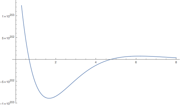
We want to find the \(e\) that will cause our \(\psi(u)\) to return values close to zero for \(u\) sufficiently far from the origin since we know that \(\psi\) should be normalizable and not blow up for large u. We can plot our differential equation at a fixed, large u (but not too large, else numerical instabilities will dominate and cause \(\psi\) to blow up anyway) as a function of our parameter \(e\). In my code, I have chosen the point \(u=10\).

Plot[pfun[e][10], {e, 0, 8}]

Plotting reveals that \(\psi(u=10, e)\) does cross the x-axis, minimizing \(\psi\) for large \(u\) at certain values of \(e\). The first such \(e\) should be our ground-state dimensionless energy. We can use FindRoot in Mathematica to determine the crossing-point to arbitrary precision. Once we find a value for \(e_0\) we can easily find \(E_0\) using our relation from before.

val = Map[FindRoot[pfun[e][10], {e, #},  WorkingPrecision -> 20] &, {2}]

Subsequent crossings of \(\psi(u=10,e)\) after the first give estimates of the values of \(e_{2n}\), the energies of the even eigenstates. If we go back to our initial conditions and realize that the first excited state in this potential will have a node at zero, we can set \(\psi(0) = 0\), \(\psi'(0) = 1\) and use the same workflow in Mathematica to find the dimensionless energies of odd eigenstates, \(e_{2n+1}\), as well. Running the full script gives \(e_0 = 0.66798655663205164945\) and \(e_1 = 2.3936438121057108370\).

These types of problems used to be particularly annoying in my MIT courses because the suggested method by the instructors was to search for the optimal value of \(e\) (to six decimal places!) by manually inputting values. Lots of time wasted because not everyone knew how to use Mathematica or of the existence of ParametricNDSolve.

The complete Mathematica code to solve this problem is copied below.

Clear[e]
pfun = ParametricNDSolveValue[{-0.5*psi''[u] + (u^4 - e)*psi[u] == 0, 
    psi[0] == 0, psi'[0] == 1}, psi, {u, -30, 30}, {e}];
Plot[Evaluate@Table[pfun[e][x], {e, 0, 1, 0.1}], {x, -10, 10}]
Plot[pfun[e][10], {e, 0, 8}]
val = Map[FindRoot[pfun[e][10], {e, #},  WorkingPrecision -> 20] &, {2}]

Regional Dialects in Germany, Austria, and Switzerland

Something that can make learning German a tiny bit confusing is the regional dialects. Sometimes people have a noticeable accent or just a different way of phrasing a common expression. Sometimes the words change entirely.

The Atlas zur deutschen Alltagssprache makes plots like those below for the usage of single words or phrase substitutions. For example, the plot below shows regional greetings in Germany, Austria, and Switzerland.

The next plot is another interesting visualization of the occurrence of city name endings (e.g. -hausen, -hof, -stadt, etc.) by location. The original plot and source code come from this site by Moritz Stefaner.

Organic Supercapacitors on Paper Substrates

Probably many people are aware of the efforts by the electronics industry to make wearable or, at least, flexible electronics. Smartphones that could be folded in half like a piece of paper and put in a pocket would certainly be desirable. Eventually, they could even be included in clothing or, rather, clothing could be included in a smartphone.

The challenge in making effective wearables and other flexible electronics is almost entirely a materials-issue: Materials must be developed to provide identical functionality as those used in modern electronics but they must also be both flexible and durable, meaning that their potency diminishes with use and repeated folding no faster than a rigid electronic device. A consumer device might need a flexible touch-display or other interface of some sort, circuit elements, and a power supply at minimum. Probably we also want some form of contactless charging too, perhaps an integrated solar cell. This is a lot of functionality to re-engineer. On top of that, some papers have explored the ambitious goal of directly printing these materials as a fully-formed device from something as simple as an inkjet printer.

I report here my work on a material that may be a potential power supply for flexible electronics on paper or textile substrates. I was responsible for the synthesis and materials characterization of PEDOT films on nylon paper substrates. This involved using oxidative chemical vapor deposition (oCVD) processes developed in Gleason Group at MIT to deposit PEDOT from monomeric EDOT. Over the course of the project I performed various tests and experiments involving thermogravimetric analysis (TGA, to observe how stable the film was), differential scanning calorimetry (DSC, also to check for stability and other thermal properties), and lots of scanning electron microscopy (SEM, to perform elemental analysis on cross-sections and check for conformal coating of the CVD layer as well as general surface morphology).

A couple interesting problems came up while working with the SEM. We wanted to perform elemental analysis using energy-dispersive x-ray spectroscopy (EDX) but we noticed that a sulfur peak (sulfur indicating the presence or lack of PEDOT) lined up with a gold peak in the spectrum making it difficult to differentiate between the two. We had to start carbon-coating our samples instead of using the standard gold-palladium sputtering to get better elemental maps like the ones in the paper. Another problem we had in getting nice images of the cross-section was that cutting our paper samples with scissors or razor blades would crush the fine mesh structure of the paper and yield poor images. We tried using a focused ion beam (FIB) with mixed results but ultimately resorted to snapping our samples in cryogenic conditions.

Here is a link to a folder containing the paper itself and the supporting information document. Please use the following citation:

Liu, Andong, Peter Kovacik, Nolan Peard, Wenda Tian, Hilal Goktas, Jonathan Lau, Bruce Dunn, and Karen K. Gleason. 2017. “Monolithic Flexible Supercapacitors Integrated into Single Sheets of Paper and Membrane via Vapor Printing.” Advanced Materials, 1606091. doi:10.1002/adma.201606091.

This work was performed at the Institute for Soldier Nanotechnologies and Gleason Lab under the supervision of Andong Liu and Karen Gleason.

Notes on Textbooks

In the physical sciences (as with other fields, I assume), there are certain texts that are considered "the classics" in that they tend to be used by the vast majority of students during their studies over multiple generations. It can take a fair amount of Internet searching or exposure to academics to figure out which books are genuine classics, so I am compiling here a tentative list of essential texts for physics and some other other topics. These recommendations are the result of my own studies and experience, recommendations from other academics, and texts used in MIT courses or recommended by students on MIT mailing lists. I will attempt to keep it updated and I have included a few notes of description (again, either from my own experience or conversations with others). Feel free to contact me if you have any additional notes or recommendations.

Electromagnetism

Jackson: Classical Electrodynamics - Treatment of Bessel function not found in most other texts, more comprehensive than Griffiths. The standard reference for classical electrodynamics.

Griffiths: Introduction to Electrodynamics - Solid introduction to electrodynamics. Used in 8.07 at MIT with some references to Jackson.

Schwinger: Classical Electrodynamics and Particles, Sources, and Fields

Quantum Optics

Wolf: Introduction to the Theory of Coherence and Polarization of Light - Brief introduction to some specialized topics.

Goodman: Fourier Optics

Mandel and Wolf: Optical Coherence and Quantum Optics - The "bible" of quantum optics.

Loudon: The Quantum Theory of Light - Offers the basics, but will need extra references for the gritty details

Glauber: Quantum Theory of Optical Coherence

XFELs

Saldin: The Physics of Free Electron Lasers

Philip Willmott: An Introduction to Synchrotron Radiation - Focus on application rather than theory, brief and to-the-point.

Quantum Mechanics

Griffiths: Introduction to Quantum Mechanics - Too brief usually, but everyone starts here.

Landau and Lifshitz: Quantum Mechanics - Non-Relativistic Theory

Quantum Field Theory

Dirac: The Principles of Quantum Mechanics

Peskin and Schroeder: An Introduction to Quantum Field Theory - Standard reference for QFT

Lifshitz: Quantum Electrodynamics

Particle Physics

Griffiths: Introduction to Elementary Particles

Quantum Chemistry

Szabo and Ostlund: Modern Quantum Chemistry - Focused on electronic structure theory
Cramer: Essentials of Computational Chemistry - Explanation and application of common models with case-studies

Jensen: Introduction to Computational Chemistry - Same as Cramer but with more focus on computational details

Craig and Thirunamachandran: Molecular Quantum Electrodynamics

Condensed Matter

Ashcroft and Mermin: Solid State Physics - The go-to reference

Altland and Simons: Condensed Matter Field Theory

Ohring: Materials Science of Thin Films

Superconductivity

Tinkham: Introduction to Superconductivity

Annett: Superconductivity, Superfluids, and Condensates

Mathematics 

Algebra:

Strang: Linear Algebra and Its Applications - Used by 18.06 at MIT

Artin: Algebra - Artin's 18.701 book is more physics-oriented than most algebra books and the chapter on representation theory is just what a physicist needs.

Dummit and Foote: Abstract Algebra

Gallian: Contemporary Abstract Algebra

Lorenzo Sadun: Applied Linear Algebra

Topology

Munkres: Topology

Differential Equations

Evans: Partial Differential Equations
Simmons: Differential Equations with Applications and Historical Notes
Strauss: Partial Differential Equations
Brauer: The Qualitative Theory of Differential Equations

Hirsch: Differential Equations, Dynamical Systems, and an Introduction to Chaos

Analysis

Rudin: Principles of Mathematical Analysis

Apostol: Calculus

Ablowitz and Fokas: Complex Variables - It's a huge book and I've only used it as a reference, but anything you might need involving complex analysis is in here somewhere.

Calculus of Variations

Geland: Calculus of Variations

Forsyth: Calculus of Variations

Mathematics in Physics

(A useful, free online resource: http://www.physics.miami.edu/~nearing/mathmethods/)
Byron and Fuller: Mathematics of Classical and Quantum Physics

Fleisch: Div, Grad, Curl and All That

Schwichtenberg: Physics from Symmetry - A really great book for introducing Lie groups and their applications to a bunch of different fields in physics.
Jeevanjee: Tensors and Group Theory for Physicists
Stillwell: Naive Lie Theory
These would be helpful for 8.033 and anything involving Lie groups, requires only 18.03 as background. They introduce the Lie stuff with a more physical and mathematical bent respectively but are written in a super casual and friendly style. In particular they staunchly avoid any differential geometry, everything here is plain old matrix multiplication.

David Skinner: Mathematical Methods - These are the lecture notes for a sophomore-level course at Cambridge. It's also relatively easy reading, requiring just 18.03; it taught me where all those weird orthogonal polynomials come from and what Green's functions are.
Zee: Group Theory in a Nutshell for Physicists - I really enjoyed Zee; it runs through a ton of group theory with minimal math prerequisites and a super casual style, showing by example. Without a proof anywhere in sight, he manages to get to grand unification in just a few hundred pages.
Schutz: Geometrical Methods of Mathematical Physics
Baez: Gauge Fields, Knots, and Gravity
Kobayashi and Nomizu: Foundations of Differential Geometry
Choquette-Bruhat and Morette: Analysis, Manifolds, and Physics
Arnold: Mathematical Methods of Classical Mechanics - A manifold underpinning of Lagrangian and Hamiltonian mechanics - less of a methods, more of a theory.
Kentaro Hori: Mirror Symmetry - The first half discusses algebraic geometry and toric geometry and I would highly recommend it if you are interested in String theory.

Plotting Transport Coefficients from BoltzTraP

BoltzTraP puts the traces of the various transport coefficient tensors (such as the conductivity tensor) in a *.trace. The trace of the conductivity tensor can be plotted using this gnuplot script. Remember to select the size to fit your display. Note that the "trace" as reported by BoltzTraP 1.2.5 is actually the trace divided by 3.

set terminal png size 2720,1800 font "Helvetica,30" linewidth 5
set output "ConductivitySym.png"
set title "Conductivity/Relaxation Time (Symmetrised)"
set xlabel "Chemical Potential (eV)"
set ylabel "1/(Ω*m*s)"

set grid

plot "data.trace" using ($1*13.605698066):6 with lines title "Conductivity/Tau"

reset

Note that this script converts the x-axis to units of electron-volts. Also remember that BoltzTraP uses the constant relaxation time approximation, so one must supply a relaxation time to get the true conductivity or mobility. The mobility is related to the conductivity by this simple formula: \(\sigma = ne\mu_e\) where \(n = N/V_{cell}\), where N is an output from BoltzTraP.

set terminal png size 2720,1800 font "Helvetica,30" linewidth 5
set output "MobilitySym.png"
set title "Mobility (Symmetrised)"
set xlabel "Chemical Potential (eV)"
set ylabel "cm^{2}/(V*s)"

set grid

set xrange [-2:2]
#Unit cell volumes in cm^3
V_cell = 10

plot "data.trace" using ($1*13.605698066):($6*tau/($3/V_cell*1.6022*10**-19)) with lines title "Mobility/Tau"

reset

Individual components of the tensors may be plotted from the corresponding file; for conductivity, this file is *.condtens.

set terminal png size 2720,1800 font "Helvetica,30" linewidth 5
set output "Conductivity_xx.png"
set title "Conductivity/Relaxation Time"
set xlabel "Chemical Potential (eV)"
set ylabel "1/(Ω*m*s)"

set grid

plot "data.condtens" using ($1*13.605698066):4 with lines title "XX",
"data.condtens" using ($1*13.605698066):5 with lines title "XY",
"data.condtens" using ($1*13.605698066):6 with lines title "XZ",
"data.condtens" using ($1*13.605698066):7 with lines title "YZ",
"data.condtens" using ($1*13.605698066):8 with lines title "YY",
"data.condtens" using ($1*13.605698066):9 with lines title "YZ",
"data.condtens" using ($1*13.605698066):10 with lines title "ZX",
"data.condtens" using ($1*13.605698066):11 with lines title "ZY",
"data.condtens" using ($1*13.605698066):12 with lines title "ZZ"

reset

As this paper points out, the effective mass can be a more useful quantity to plot from calculations because conductivity/mobility are dependent on the scattering time and mix knowledge of the electronic structure (which, in principle, we know from the DFT calculation) and the scattering properties of the material and its carriers (which we probably do not know at all). The effective mass is, in this sense, more useful because it gives information about the electronic structure without requiring any knowledge of scattering in the material. The paper gives the formula \(m^* = \frac{e^2 \tau |N|}{\sigma V_{cell}}\) where \(\tau/\sigma\) is the reciprocal of an output from BoltzTrap. \(N\) is another output from BoltzTraP in the *.trace file.

set terminal png size 2720,1800 font "Helvetica,30" linewidth 5
set output "MassSym.png"
set title "Effective Mass"
set xlabel "Chemical Potential (eV)"
set ylabel "Mass in m_{e}"

set grid

set xrange [-2:2]
#Unit cell volumes in m^3
V_cell = 10

# tau = 10**-12 #Guess relaxation time
# sigma = n * e * mu
# 1/m = sigma/(e**2 * tau) * 1/n
# n = abs(N)/V_cell
# Checked, relations used below have proper units of mass

plot "data.trace" using ($1*13.605698066):(abs($3)/V_cell*(1.602177*10**-19)**2/$6)/(9.1093836*10**-31) with lines title "Mass"

reset

N.B.: Do not trust WolframAlpha to correctly convert cubic Angstroms to cubic centimeters!

References

Gibbs, Zachary M., Francesco Ricci, Guodong Li, Hong Zhu, Kristin Persson, Gerbrand Ceder, Geoffroy Hautier, Anubhav Jain, and G. Jeffrey Snyder. 2017. “Effective Mass and Fermi Surface Complexity Factor from Ab Initio Band Structure Calculations.” npj Computational Materials. Springer US: 1–6. doi:10.1038/s41524-017-0013-3.

A Java Calculator for Oxide Growth

I created this Java applet while employed as a high school intern at Rogue Valley Microdevices (RVM). I was a lab tech in the foundry and we used a calculator on RVM's website to calculate our run times for the oxide furnaces. This proved problematic one week when, for some reason, the Internet connection in the lab kept cutting out (plus, the website was just slow sometimes). I created this applet so we would not have to rely on a good Internet connection and it was used for a few years at RVM (last time I asked about this was around a year ago, I think). This program also proved useful later in a class at MIT where we were given the pointless task of calculating oxide growth times by hand in a problem set. It was also the first time I had created something that was useful in "the real world".

You can download the .jar file here. Please attribute my code if you use it in your own work. Below is a screenshot of the interface.

I owe a lot to RVM and the skills they taught me. The knowledge I acquired there helped me get my first research internship at MIT in Karen Gleason's group working on organic CVD and polymeric conductors.

Quantum Espresso Molecular Dynamics Animation

I've been using Quantum Espresso for some projects and I created this animation using XCrySDen on a molecular dynamics relaxation job I ran. It is a fairly interesting animation: One can make out many of the vibrational modes in the molecule, particularly those of the hydrogen atoms (light blue), even though this was not the goal I had in mind. Sometimes using the method with the least sophistication can still produce some insight into the physics or at least make some fun animations.

In quantum chemistry, the first step of most simulations will be to "relax" a molecular structure; this means to search the potential energy surface to find the minimal energy structure (i.e., the most stable structure). The relaxed structure is assumed to be an accurate model of the physical compound. Higher quality relaxations, typically those using a higher level of theory such as perturbation or coupled-cluster, make for a more realistic geometry, in principle. However, higher quality always translates to more "expensive" which, in scientific computation, refers to the amount of resources (time and computational hardware, usually) one must throw at a particular simulation.

Molecular dynamics is regarded as a very "cheap" method because it does not use an algorithm to search the energy landscape for a path to the minimal energy structure. Instead, the straight-forward approach of molecular dynamics is to integrate the forces applied to each atom directly using something like a Verlet or damped-Newtonian model. This is mathematically inefficient since you might not converge to the minimal energy very quickly but the method is computationally "cheap" so it is a good starting point, especially if you know your initial structure is very far from the correct geometry as I assumed for my calculation: Algorithms like conjugate gradient or BFGS are only most efficient when the structure is already close to a minimum in the energy landscape.

There is a lot more to be said about structure relaxation, the theory and the best way to do it in practice, and vibrational modes but I will leave that for another time.

Muting the Startup Tone in OSX

This is a hack that I have found infinitely useful due to the amount of annoyance it saves. No one appreciates the person who comes to a lecture (maybe a few minutes late), opens their MacBook, hits the power button, and treats everyone to the Mac startup tone at full volume. This method ensures this will never happen again. Sadly, I do not remember now where I first read it as it was some years ago.

The idea is to create two scripts, one that mutes and one that unmutes: When the Mac is shut down, one script mutes the system so that the next startup will not produce the tone and the second script unmutes the system at login (following the usual occurrence of the tone, which happens at startup but before login) so that the system functions as normal.

Below, the contents of mute-on.sh

#!/bin/bash
osascript -e 'set volume with output muted'

Below, the contents of mute-off.sh

#!/bin/bash
osascript -e 'set volume without output muted'

Put these two scripts in a location of your choosing and run the following to create the appropriate Login Hooks

sudo chmod u+x /Library/Scripts/mute-on.sh
sudo chmod u+x /Library/Scripts/mute-off.sh
sudo defaults write com.apple.loginwindow LogoutHook /Library/Scripts/mute-on.sh
sudo defaults write com.apple.loginwindow LoginHook /Library/Scripts/mute-off.sh

To remove the Login Hooks so you can hear the login tone again

sudo defaults delete com.apple.loginwindow LoginHook
sudo defaults delete com.apple.loginwindow LogoutHook

One deficiency with this hack that I've noticed is that when one uses the headphone jack and shuts down the system with the plug still in the jack (removing the plug after shutdown) sometimes the next startup will produce the hated tone. This effect is rare enough though (I do not think it happens every time) that I have not bothered to try and find a further solution.

Fourier Transform Miscellanea

The Fourier Transform in Circular Symmetries

The Bessel equation of the first-kind, zero order is defined as
    \begin{equation}
        J_0(a) = \frac{1}{2\pi} \int_{0}^{2\pi} e^{-ia \cos(\theta - \phi)} d\theta
    \end{equation}
We thus define the Fourier Transform
    \begin{equation}
        G_0(\rho, \phi) = G_0(\rho) = 2\pi \int_{0}^{\infty} r g(r) J_0(2\pi r \rho) d\rho
    \end{equation}
and its inverse transform
    \begin{equation}
        g(r) = 2\pi \int_{0}^{\infty} \rho G_0(\rho) J_0(2\pi r \rho) d\rho
    \end{equation}
  

Discretizing the Fourier Transform

Discretizing the Fourier Transform allows us to use the Fast Fourier Transform (FFT) to quickly acquire the Fourier Transform of a continuous function in Python.

Discretize time and frequency
    \begin{equation}
        t = m\Delta t + t_0 \qquad
        \omega = k \Delta \omega \qquad
        \Delta t \Delta \omega = \frac{2 \pi}{N}
    \end{equation}
where \(m,k \in \mathbb{Z}\) and \(N\) is the number of samples. Using the definition of the Fourier Transform
    \begin{equation}
           F(\omega) = \frac{1}{\sqrt[]{2\pi}} \int_{-\infty}^{\infty} e^{-i\omega t} f(t) dt
    \end{equation}
we can substitute the previously defined quantities to get
    \begin{align}
        F(k\Delta \omega) &\approx \frac{1}{\sqrt[]{2\pi}} \sum_{m=1}^{N} \Delta t f(t_0 + m\Delta t) e^{-i k \Delta \omega (t_0+m\Delta t)} \\&= \frac{1}{\sqrt[]{2\pi}} \Delta t e^{-i t_0 k \Delta \omega} \sum_{m=1}^{N} e^{-2\pi i \frac{mk}{N}} f(t_0 + m\Delta t)
    \end{align}
Now notice that, in the final result, the constant phase factor is being multiplied by the discrete Fourier Transform (DFT) on the right. We may now use the FFT to calculate the DFT, keeping in mind that we must multiply by the phase factor to get an approximation of the continuous Fourier Transform.

We can define the inverse transform in exactly the same way
    \begin{equation}
        \omega = n \Delta \omega + \omega_0 \qquad
        t = l \Delta t \qquad
        \Delta t \Delta \omega = \frac{2 \pi}{N}
    \end{equation}
where \(n,l \in \mathbb{Z}\) and \(N\) is defined as before. Now the inverse transform is
    \begin{equation}
           f(t) = \frac{1}{\sqrt[]{2\pi}} \int_{-\infty}^{\infty} e^{i\omega t} F(\omega) dt
    \end{equation}\begin{align}
        f(l \Delta t) &\approx \frac{1}{\sqrt[]{2\pi}} \sum_{m=1}^{N} \Delta \omega F(\omega_0 + n\Delta \omega) e^{-i l \Delta t (\omega_0+n\Delta \omega)} \\&= \frac{1}{\sqrt[]{2\pi}} \Delta \omega e^{-i \omega_0 l \Delta t} \sum_{m=1}^{N} e^{-2\pi i \frac{nl}{N}} F(\omega_0 + n\Delta \omega)
    \end{align}

Python Code

This code works well for messing around with Fourier Transforms.

import numpy as np
import matplotlib.pyplot as plt
import scipy.fftpack

# Number of samplepoints
N = 600
# sample spacing
T = 1.0 / 800.0
x = np.linspace(0.0, N*T, N)
y = np.sin(50.0 * 2.0*np.pi*x) + 0.5*np.sin(80.0 * 2.0*np.pi*x)
yf = scipy.fftpack.fft(y)
xf = np.linspace(0.0, 1.0/(2.0*T), N/2)

fig, ax = plt.subplots()
ax.plot(xf, 2.0/N * np.abs(yf[:N//2]))
plt.show()

Friedel's Law

Given a real function, its Fourier transform \begin{equation} F(k) = \int_{-\infty}^{\infty} f(x) e^{ikx} dx \end{equation} has the following properties. 

• \(F(k) = F^*(-k) \)
• \(|F(k)|^2 = |F(-k)|^2\)
• The phase of F, however, is antisymmetric: \(\phi(k) = -\phi(-k)\)

Centrosymmetric points \((k, -k)\) are called Friedel or Bijvoet pairs.

Correcting Coherent Errors with Surface Codes

Update (31.10.18): This project was recently published in Nature!

This is a paper that resulted from a project I assisted with during a summer internship with the group of Robert König at TU München. I was responsible for writing efficient C++ code to simulate the algorithms proposed in the paper. I cannot claim to understand all of the mathematics involved but I thought the code I wrote worked pretty well. I was also grateful for the opportunity to sample the academic environment in Germany.

Here is a link to our paper on the arXiv. The abstract is copied below.

"We study how well topological quantum codes can tolerate coherent noise caused by systematic unitary errors such as unwanted Z-rotations. Our main result is an efficient algorithm for simulating quantum error correction protocols based on the 2D surface code in the presence of coherent errors. The algorithm has runtime O(n2), where n is the number of physical qubits. It allows us to simulate systems with more than one thousand qubits and obtain the first error threshold estimates for several toy models of coherent noise. Numerical results are reported for storage of logical states subject to Z-rotation errors and for logical state preparation with general SU(2) errors. We observe that for large code distances the effective logical-level noise is well-approximated by random Pauli errors even though the physical-level noise is coherent. Our algorithm works by mapping the surface code to a system of Majorana fermions."

Water Molecular Dynamics - Some Graphs

I made these plots a few years ago for a class on quantum chemical simulation at MIT; I still find them interesting to look at sometimes. These plots were produced from a molecular dynamics simulation with magnesium chloride in an explicit water solvent using various water models such as TIP3P/TIP4P and SPCFW.

You will notice that the quantities plotted below have wildly fluctuating raw data due to the small number of explicit solvent molecules present in the simulation. How is this useful? The point here is that the averages of these quantities stabilize and reach equilibrium by the end of the simulation. Molecular dynamics simulations frequently makes use of the ergodic hypothesis in this way.

Each plot includes the raw data, a smoothed version of the raw data, and a cumulative average. For experimentalists, it is usually only the average at the end of simulation that is important as this is assumed to be the equilibrium value of the measured quantity.

Water density (no solute) over time in the SPCFW model.

Water temperature (no solute) over time in the SPCFW model.

Water temperature (no solute) over time in the SPCFW model.

Radial probability distribution of water molecules around magnesium and chloride ions in solution. Note the secondary water shell of magnesium.

Distance between magnesium ion and both accompanying chloride ions over time in solution. 

Heilmeier's Catechism

This is a set of questions that I was unaware of until one of my professors at MIT mentioned it in a class. It's a good rubric for any project and I'm not sure why it is not more commonly known. Or perhaps it is and I'm just the last person to learn about it.

From the Wikipedia page: A set of questions credited to George H. Heilmeier that anyone proposing a research project or product development effort should be able to answer.

• What are you trying to do? Articulate your objectives using absolutely no jargon.
• How is it done today, and what are the limits of current practice?
• What's new in your approach and why do you think it will be successful?
• Who cares? If you're successful, what difference will it make?
• What are the risks and the payoffs?
• How much will it cost?
• How long will it take?
• What are the midterm and final "exams" to check for success?

Good questions to come back to on any serious project or research.

Mathematica Basic Functions and Examples

Reading software documentation is boring and Mathematica is a pain so here are some examples of the key functions and their syntax just to get started. I will attempt to update this in the future although I try to find alternatives to Mathematica whenever possible.

# Integration
Integrate[2*Sqrt[2]/(3*a)*x*Sin[2*Pi*x/a]*Sin[3*Pi*x/a], {x, 0, a}]

# Numerical Integration
N[Integrate[4/a^3*r^2*Exp[-2 r/a], {r, 0, a/53600}]]

# Integration over multiple dimensions
Integrate[1/(2*u)*(Q*w*u/(4*Pi*R))^2*((1 - 3*r^2/(5*R^2))^2*Cos[t]^2 + 
(1 - 6*r^2/(5*R^2))^2*Sin[t]^2)*r^2*Sin[t], {t, 0, Pi}, {p, 0, 2 Pi}, {r, 0, R}]

# Finding Intersections
pts = NSolve[x*Cot[x] == -y*Coth[y] && {x, y} \[Element] Circle[{0, 0}, 2*Pi], {x, y}]

# A plot of the above intersections
ContourPlot[{x*Cot[x] + y*Coth[y] == 0 , x^2 + y^2 == 4 Pi^2}, 
{x, -4 Pi, 4 Pi}, {y, -4 Pi, 4 Pi}]

# The Quantum Harmonic Oscillator and some expectation values
Clear[m, \[Omega], \[HBar], n];
(*m=1*)
(*\[Omega]=1*)
(*\[HBar]=1*)

psi[x_, n_] := (m*\[Omega]/(Pi*\[HBar]))^(1/4)*1/Sqrt[2^n*n!]*
  HermiteH[n, Sqrt[m*\[Omega]/(\[HBar])]*x]*
  Exp[-m*\[Omega]*x^2/(2*\[HBar])]
En[n_] = \[HBar]*\[Omega]*(n + 1/2)
En[0]
psi[x_, t_, n_] := (m*\[Omega]/(Pi*\[HBar]))^(1/4)*1/Sqrt[2^n*n!]*
  HermiteH[n, Sqrt[m*\[Omega]/(\[HBar])]*x]*
  Exp[-m*\[Omega]*x^2/(2*\[HBar])]*Exp[-i*En[n]*t/\[HBar]]
psi[x, 0]
psi[x, t, 0]
expX[n_] := Integrate[x*psi[x, n]^2, {x, -Infinity, Infinity}]
expX2[n_] := Integrate[x^2*psi[x, n]^2, {x, -Infinity, Infinity}]
DeltaX[n_] := Sqrt[expX2[n] - expX[n]^2]

# Expand expressions
Expand[Sum[
  1 + e^(I*(Subscript[K, 3] - Subscript[K, 1]) (Subscript[x, i] - 
        Subscript[x, k])) + 
   e^(I*(Subscript[K, 1] - Subscript[K, 2]) (Subscript[x, j] - 
        Subscript[x, i])) + 
   e^(I*(Subscript[K, 2] - Subscript[K, 3]) (Subscript[x, k] - 
        Subscript[x, j])) + 
   e^(I*(Subscript[K, 1]*(Subscript[x, j] - Subscript[x, i]) + 
        Subscript[K, 2]*(Subscript[x, k] - Subscript[x, j]) + 
        Subscript[K, 3]*(Subscript[x, i] - Subscript[x, k]))) + 
   e^(I*(Subscript[K, 1]*(Subscript[x, k] - Subscript[x, i]) + 
        Subscript[K, 2]*(Subscript[x, i] - Subscript[x, j]) + 
        Subscript[K, 3]*(Subscript[x, j] - Subscript[x, k]))), {i, 
   n}, {j, n}, {k, n}]]

# Simplify expressions, '%' uses the result of the previous input
FullSimplify[%]

A couple key differences to note about Mathematica: The use of square brackets instead of parentheses to contain arguments to functions, function names are capitalized, comments are indicated by '(*' and a closing '*)', and user-defined functions are created using ':=' and underscores on any arguments. If possible, I encourage use of open source alternatives such as Octave or Python. However, I have to admit that, when it comes to getting integration and algebra of complicated expressions done quickly, nothing beats Mathematica.

Using Wine for Gaming in OSX - SWTOR

I like Star Wars and sometimes I feel compelled to revisit the games from my youth; however, this can be a bit difficult when one uses OSX (though there are some excellent ports of the classics, and other favorites, from Aspyr Media on the App Store). Wine, again, proves to be very useful in this area even for the MMORPG Star Wars The Old Republic at the highest graphics settings.

Setup for this game requires some patience but not nearly so much as it used to be when the clues were more scattered a few years ago (plus there are fewer steps required now, for a number of reasons). This guide on reddit is kept up-to-date and is very comprehensive but I'll describe what I did for reinforcement.

Download the latest Wine Staging version. I have had problems trying to use MacPorts to install Wine so I recommend downloading the installer from the website directly. 

Open a Terminal using your Wine install. Use "winecfg" to set Windows 10, and include d3dx9_43, crypt32. Remember, the default is that all Wine related items are stored in a mock Windows-style directory tree in ~/.wine. This is where all of the SWTOR files will be installed.

Download and run the SWTOR installer with Wine. I have only tested the "Express" install and had no issues with this step.

Run the SWTOR launcher by changing into the install directory under ~/.wine. Then, login to your account. At this point, an error will popup saying something about administrative privileges. Close the launcher. Open launcher.settings using a text editor and change the line "bitraider_disable": false to "bitraider_disable": true.

Run the launcher again. Login and allow the game to patch. Expect this to take several hours depending on your connection. The full game is 38 GB on the hard drive so make sure you can afford the space.

Screen shot of launcher window on OSX

Once you are fully patched, that should be it. I have played the game a couple of times since installing and it runs well even over WiFi on the highest graphics settings. I'm sure using Wine to run other Windows games on OSX would work well too. My MacBook has an AMD Radeon R9 M370X in addition to the integrated Intel Iris Pro so your mileage may vary on your own system. 

May the Force be with you.

Compiling BoltzTraP 1.2.5 on OSX

Update (21.6.18): I've noticed in using BoltzTraP2 that it has much greater numerical stability than previous versions of BoltzTraP. I must conclude that BoltzTraP2 gives much more reliable results. Reproducing the band structure near band crossings, as I mentioned previously, may be failing due to insufficient k-point sampling in terms of overall density at specific locations in k-space that are required to resolve the bands near a crossing.

Update (19.6.18): I was not unaware of BoltzTraP2, but I was skeptical of the new version at first (and I was determined to get 1.2.5 working again). Turns out, it works rather well and is easy to use without the need to write custom scripts for converting or processing data from an electronic structure code output. It also allows interactive plotting of the entire Fermi Surface which is a fun feature. The transport coefficients calculated are nearly identical to those calculated in version 1.2.5 and the built-in plotting feature facilitates plotting over a range of temperatures.

Fermi surface of silicon as calculated from VASP in BoltzTraP2. 

Another section of the silicon Fermi surface.

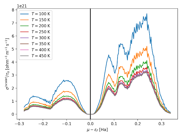
Conductivity of silicon as a function of chemical potential at various temperatures as calculated in BoltzTraP2.

Conductivity of silicon as calculated in BoltzTraP 1.2.5. Roughly corresponds to the region between -0.1 and 0.1 Hartrees in the previous plot. The point is just to show that the main features are reproduced with identical orders of magnitude.

The plotting tool is not, however, great for plotting band structures: It does not give the smooth plots that can be made in Python and often gets confused near band crossings. I suspect that this is probably an issue with the plotting function itself and not due to the interpolation, which the BoltzTraP team claimed in their original paper sufficiently approximated the band structure near band crossings for the purpose of calculating the transport coefficients.  

Band structure of silicon from VASP plotted using custom data processing and scripts.

Band structure of silicon plotted by BoltzTraP2 across the same high symmetry points as in the previous plot. Note here, however, that the features are not reproduced with the same resolution nor even with the same accuracy near band crossings. BoltzTraP2 does give a rough idea of the features but clearly it is necessary to do a full band structure calculation with explicit k-point path in VASP rather than interpolate a uniform k-point density DOS calculation as BoltzTraP2 does. 

Follow this tutorial for more information. I tested it using VASP calculations on silicon and had no problems.

Original: I recently had some trouble getting BoltzTraP to compile and play nicely with MacPorts so I am posting the final results. It is the upper section of the Makefile that is most important but I have included the entirety for completion. I used MacPorts' gfortran, lapack (+gfortran), and scalapack (+gfortran). It proved important to not let the compiler or linker find any ATLAS libraries or OSX's Accelerate framework: If you have ATLAS installed through MacPorts, there will be a liblapack.a in /opt/local/lib that belongs to ATLAS. The Makefile below correctly tells the linker to use /opt/local/lib/lapack instead.

# BoltzTraP 1.2.5 Makefile

SHELL = /bin/sh
FC = /opt/local/bin/gfortran
FOPT  = -g -funroll-loops -O3 -ffast-math -fgcse-lm -fgcse-sm -ffast-math \
-ftree-vectorize -fexternal-blas -fleading-underscore -g -p -pg -Wall \ 
-fbounds-check -finit-integer=-666 -finit-real=nan

LDFLAGS = -L/opt/local/lib/lapack -L/opt/local/lib/
LIBS = -lblas -lscalapack -llapack

LINKER = $(FC)
DESTDIR = .
EXECNAME = BoltzTraP

###############################################################################

FFLAGS = $(FGEN) $(FOPT)
EXEC = $(DESTDIR)/$(EXECNAME)

#..............................................................................
#
#  Object files common to both REAL and COMPLEX type subroutines
#
OBJS = gmlib2.o reallocate.o \
     m_bandstructure.o m_input.o m_fermimod.o \
     m_interfaces.o \
     latgen2.o generic_field.o gtfnam.o gen_lattpoints.o \
     BoltzTraP.o crystal_band.o wien_band.o phon_band.o generic_band.o pw_interface.o \
     add_inv.o bandana.o stern1.o kdelta.o fite4.o sortag.o gplbands.o \
     dos.o ifflim.o setfft.o c3fft.o boseintegrals.o fermiintegrals.o bands.o kcomp.o \
     bz.o fermisurface.o setfft2.o write_dx_fs.o write_dx_bz.o write_cube_fs.o \
     dos_histogram.o dos_tetra.o noculc.o dosvv.o readvv.o \
     phonondrag.o
#OBJS = \
#        reallocate.o defs.o modules.o broad.o add_inv.o \
#        c3fft.o gtfnam.o ifflim.o mknam.o read_energy.o \
#        transport.o stern.o kdelta.o gen_lattpoints.o fite4.o setfft.o \
#        starfkt2.o dos.o 

$(EXEC): $(OBJS)
 $(LINKER) $(LFLAGS) -o $(EXEC) $(OBJS) $(LDFLAGS) $(LIBS) $(LFLAGS)


clean:
 rm -f *.o *.mod *.pc *.pcl *~

.SUFFIXES: .F90 .o 
.F90.o:
 $(FC) $(FFLAGS) -c $<

OpenCL with C++ Bindings in XCode

I've recently started learning OpenCL for my work at DESY CFEL and found that setting up a C++ environment in XCode for OpenCL is not an entirely straightforward task. Here are some instructions to get started. I am using OSX 10.13.4 (High Sierra) and XCode 9.3.1.

The OpenCL framework in OSX is stored at /System/Library/Frameworks/OpenCL.framework/. Unfortunately, it does not come with a header file for C++ bindings; if you want to use C alone this should not be a problem. I would like to use C++, however.

Download the appropriate cl.hpp file from the Khronos OpenCL Registry. Simply add and include this header file in XCode OpenCL projects and it should work fine. Do not forget to actually link the OpenCL framework under the project settings in XCode. Download and compile this example code, mostly copied from this tutorial, to test your system.

It is possible to add cl.hpp to the system framework so that you do not have to manually add it every time you create a new project. There is one complication: Since OSX 11.11 (El Capitan), Apple has started using something called System Integrity Protection (SIP) to prevent the naive or overly-adventurous from doing too much damage. When activated, it will prevent adding the header to the OpenCL framework even with root access.

This page provides the solution. Restart your system and hold cmd+R to launch OSX in Recovery Mode. Open a Terminal and enter csrutil disable to disable SIP. Restart normally. Move your cl.hpp file to /Applications/Xcode.app/Contents/Developer/Platforms/MacOSX.platform/Developer/SDKs/MacOSX.sdk/System/Library/Frameworks/OpenCL.framework/Headers. Return to Recovery Mode and enter csrutil enable in a Terminal if you wish to reenable SIP and restart again. You should now be able to include <OpenCL/cl.hpp> in all of your XCode OpenCL projects.

Notice here that, despite the fact that OpenCL has been released up to version 2.2 as of 2018, Apple devices come with drivers only up to version 1.2. Additionally, it is impossible (as far as I know) for users to update these drivers in OSX. Clearly, Apple has no interest in providing sufficient support for OpenCL. This is due to Apple's development of its Metal framework which, in their eyes, is the obvious choice for anyone developing for the GPU in OSX. Personally, I have no interest in learning an API that is only useful for one system so I hope this is rectified in the future.

References:
Khronos Group
Apple Developer OpenCL Programming Guide for Mac

Using PowderCell to Calculate Angles for Debye-Scherrer Cones

PowderCell is a piece of software that allows calculation of the polar angles of the Debye-Scherrer cones in x-ray powder diffraction. We used these angles to find the alignment of the photon detectors in the experiment I mentioned in a previous post. We used the predicted powder scattering angles from PowderCell, projected them onto a simulated flat detector, and moved the detector in the program until the experimental powder rings lined up with the predicted powder rings. Here is a short tutorial for how to calculate these angles in PowderCell.

Using Wine to Run Windows Programs

PowderCell is a Windows program, but we can still run it in OSX using a cool piece of software called Wine. The short story of Wine is that it will allow you run any Windows software natively in OSX --- no dual-booting Windows necessary! I used to have a Windows partition on my Mac but now I use Wine instead: It is much more convenient works well for running all sorts of programs including your favorite Windows video games.

You can install Wine on OSX through a number of different methods; I have had success with installing the downloadable binaries and installing through MacPorts and Homebrew. Currently, I am using the MacPorts version.

The first time you start up Wine, it will create a hidden directory, ~/.wine,  in ~/ where it will store all of Windows files and programs you will run. The directory structure roughly mimics Windows with directories called drive_c, Program Files, Application Data, and all the other classics more or less in the place you expect. If you ever mess with the directory structure and break things just delete the entire ~/.wine directory and reinstall all of your programs, it will not break anything related to OSX. Installation of programs works just like it would in Windows.

Run Windows programs with Wine by running

wine program.exe

Some other important commands that allow you to change various settings such as which Windows version you are running as

winecfg
wine regedit

Using PowderCell 2.4

Download PowderCell and run it using Wine. It will ask to extract all of the necessary files to a location of your choosing. After extraction, move to the new directory and run PCW.exe, again with Wine. Some additional comments about running PowderCell with Wine are here.

Now that we have the program running, let's calculate something. In the experimental setup featured in my previous post, we performed x-ray diffraction on powdered lanthanum hexaboride using the LINAC Coherent Light Source at the Stanford Linear Accelerator Laboratory. First, we must download a unit cell .cif file for \(LaB_6\) using the Crystallography Open Database or any other crystallography database your institution gives access to.

PowderCell is an old program and will, unfortunately, not read the .cif file directly. Simply open the unit cell in a text editor and enter the unit cell data manually as pictured below. Be sure to enter the space group correctly. The space group number for \(LaB_6\) is 221. A visualization of your unit cell should automatically be generated after pressing "OK".

In our experiment last month, we used x-rays with energy of 9.43 keV which corresponds to a wavelength of 1.315 angstroms. Under Diffraction >> Experiment, make sure the source is "X-ray" and enter the wavelength in angstroms for your source in the field \(K\alpha_1\). In this window you can also change the range of viewing angles. The peaks of the Debye-Scherrer cones will automatically be plotted for your structure.

The option to view the numerical angles, \(2\theta\), printed above the peaks is given in the right-hand column.